Predicting Hotel Booking Cancellations Using Machine Learning With Python
Booking cancellations have a substantial impact on demand management decisions in the hospitality industry.
Every year, more than 140 million bookings were made on the internet and many hotel bookings were booked through top-visited travel websites like Booking.com, Expedia.com, Hotels.com, etc.

Hotel Booking Cancellations, A Growing Problem…
When Analyzing the past 5 years data, D-Edge Hospitality solutions has found that the global average cancellation rate on bookings has reached almost 40% and this trend produces a very negative impact on hotel revenue.

To overcome the problems caused by booking cancellations, hotels implement rigid cancellation policies, inventory management, and overbooking strategies, which can also have a negative influence on revenue and reputation.
Once the reservation has been canceled, there is almost nothing to be done and it creates discomfort for many Hotels and Hotel Technology companies. Therefore, predicting reservations which might get canceled and preventing these cancellations will create a surplus revenue for both Hotels and Hotel Technology companies.
Motivation
Have you ever wondered what if there was a way we could predict which guests are likely to Cancel the Hotel Booking? That would be great right?
Luckily, by using Machine learning with Python, we can predict the guests who are likely to cancel the reservation at the Hotels and this will create a surplus revenue, better forecasts and reduce uncertainty in business management decisions.
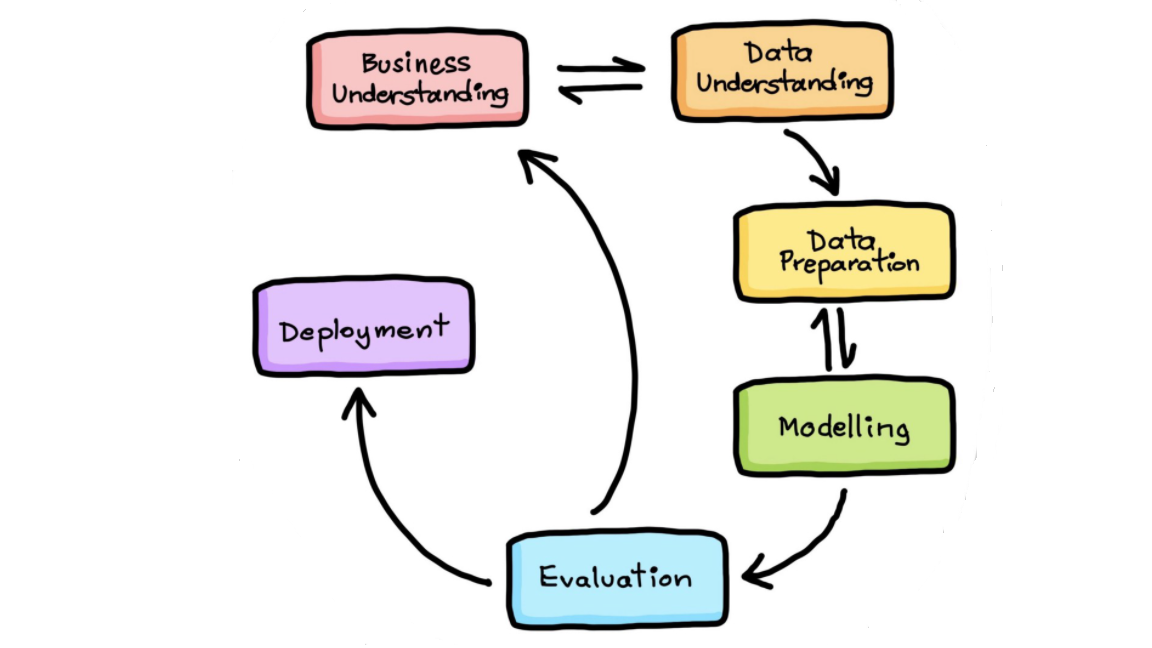
If you want to follow a process while working on a machine learning project, this blog is for you. In this blog, I will walk you through the entire process of solving a real-world Machine learning project right from understanding the Business problem to the Model deployment on the cloud.
Machine Learning Project Life Cycle
- Understanding the Business Problem
- Data Collection and Understanding
- Data Exploration
- Data Preparation
- Modeling
- Model Deployment
1. Understanding Business Problem
The Goal of this project is to Predict the Guests who are likely to Cancel the Hotel Booking using Machine Learning with Python. Therefore, predicting reservations which might get canceled and preventing these cancellations will create a surplus revenue, better forecasts and reduce uncertainty in business management decisions.
2. Data Collection and Understanding
This dataset contains booking information for a City hotel and a Resort hotel, and includes information such as when the booking was made, length of stay, the number of adults, children, and/or babies, and the number of available parking spaces etc.
I have collected the dataset from the kaggle. Dataset is available at Kaggle Dataset
3. Data Exploration
In this step, we will apply Exploratory Data Analysis (EDA) to extract insights from the data set to know which features have contributed more in predicting Cancellations by performing Data Analysis using Pandas and Data visualization using Matplotlib & Seaborn. It is always a good practice to understand the data first and try to gather as many insights from it.
Below are tasks to be performed:
- What is MongoDB Atlas Cloud?
- Steps to setup MongoDB Atlas Cloud
- Importing Libraries
- Storing the data into MongoDB Atlas Cloud Database
- Loading (Fetching) data from MongoDB Atlas Cloud Database
- Exploratory Data Analysis (EDA) on all Features
- Data Visualisation on all Important Features
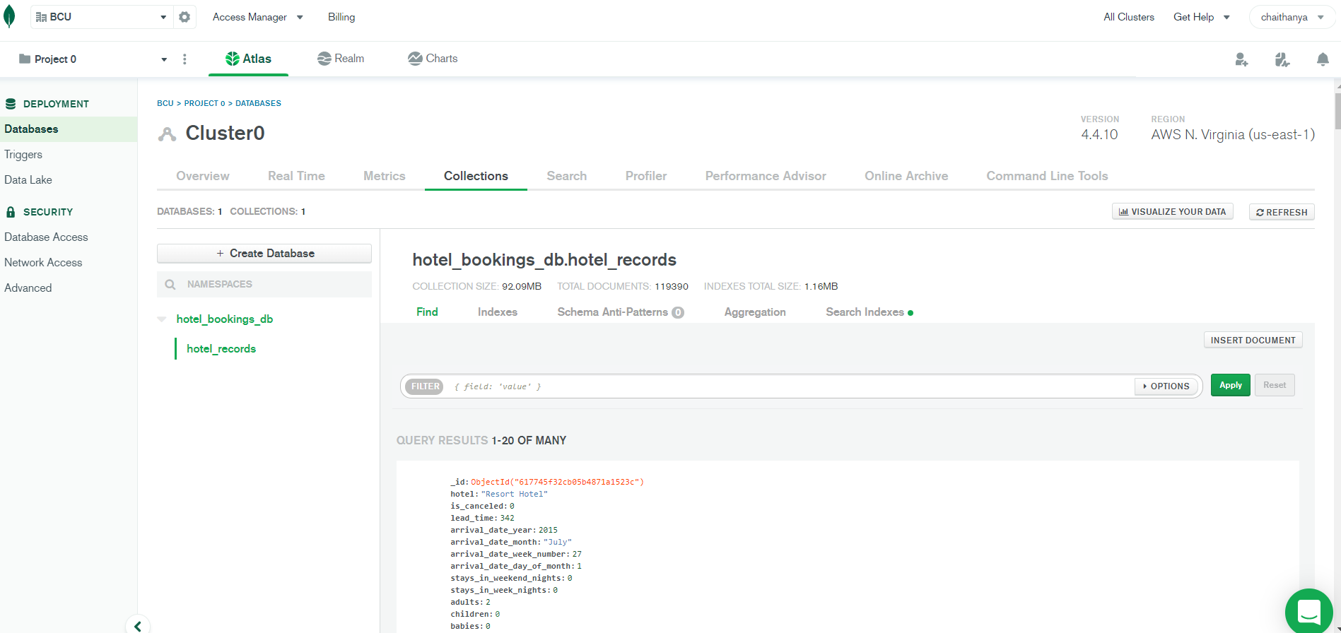
3.1 What is MongoDB Atlas Cloud?
MongoDB Atlas is a fully-managed Database-as-a-Service (DBaaS) cloud database that handles all the complexity of deploying, managing, and healing your deployments on the cloud service provider of your choice (AWS , Azure, and GCP). MongoDB Atlas is the best way to deploy, run, and scale MongoDB in the cloud.
In this project, we will store the dataset into MongoDB Atlas cloud database by following industry best practices which helps in managing the data in scalable, robust and secure manner.
3.2 Steps needed to get started using MongoDB Atlas Cloud:
1. Create an Atlas Account using Gmail Id
2. Create a Free Cluster in MongoDB Atlas Cloud

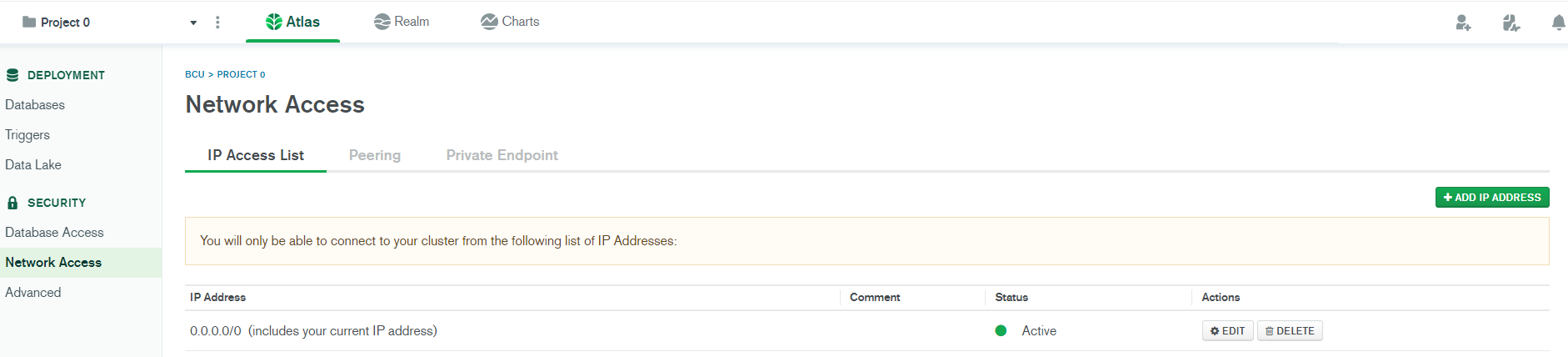
3. Add Your Connection IP Address to Your IP Access List
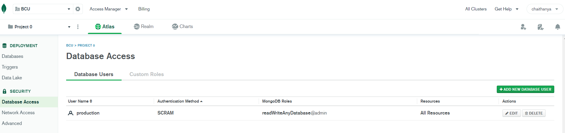
4. Create a Database and User for Your Cluster with username and password to make it secure
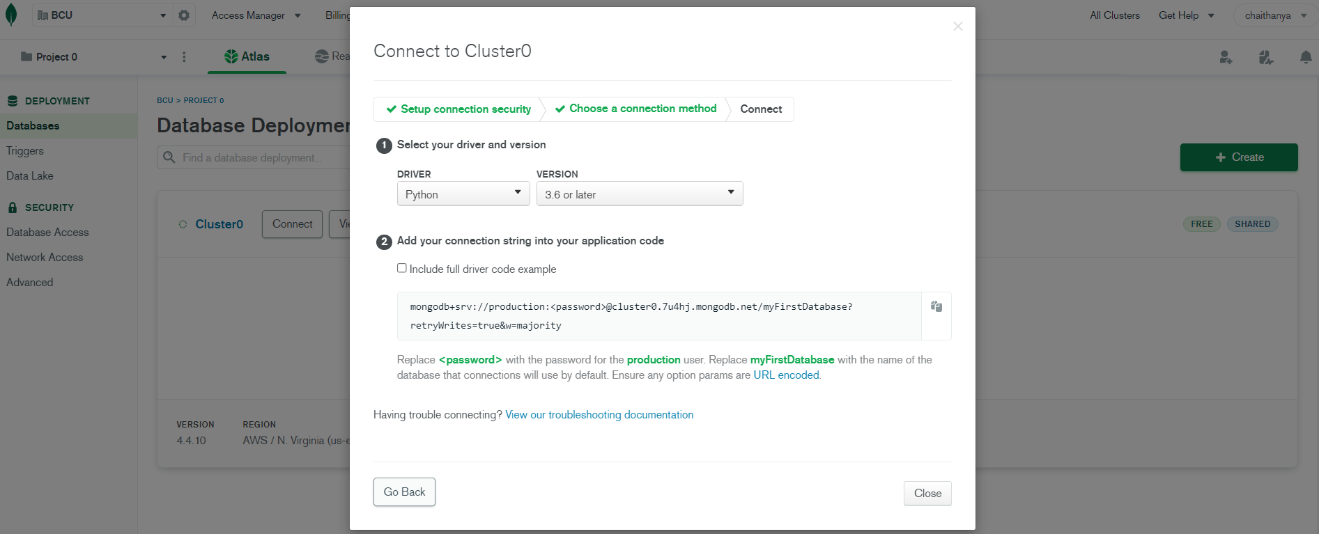
5. Connect to Your Cluster
6. Insert and View Data in Your Cluster
3.3 Importing Libraries
import pandas as pd
import numpy as np
import matplotlib.pyplot as plt
%matplotlib inline
plt.figure(figsize=(12,6))
import seaborn as sns
from warnings import filterwarnings
filterwarnings('ignore')
<Figure size 864x432 with 0 Axes>
3.4 Storing the Dataset into MongoDB Database
# Install and import Pymongo libraries to connect with MongoDB Atlas Cloud
!pip install pymongo
!pip install 'pymongo[srv]'
!pip install dnspython

from pymongo import MongoClient
Requirement already satisfied: pymongo in /usr/local/lib/python3.7/dist-packages (3.12.0)
Requirement already satisfied: pymongo[srv] in /usr/local/lib/python3.7/dist-packages (3.12.0)
Requirement already satisfied: dnspython<2.0.0,>=1.16.0 in /usr/local/lib/python3.7/dist-packages (from pymongo[srv]) (1.16.0)
Requirement already satisfied: dnspython in /usr/local/lib/python3.7/dist-packages (1.16.0)
# Establish a connection to a MongoDB Atlas Cluster with Secured Authentication using User Name and Password of the Database
client = MongoClient("mongodb+srv://production:prod_db@cluster0.7u4hj.mongodb.net/myFirstDatabase?retryWrites=true&w=majority")
# Create Database and specify name of database
db = client.get_database('hotel_bookings_db')
# Create a collection
records = db.hotel_records
# Create Dataframe and Read the dataset using Pandas
df = pd.read_csv('/content/bookings.csv')
df.head()
| hotel | is_canceled | lead_time | arrival_date_year | arrival_date_month | arrival_date_week_number | arrival_date_day_of_month | stays_in_weekend_nights | stays_in_week_nights | adults | children | babies | meal | country | market_segment | distribution_channel | is_repeated_guest | previous_cancellations | previous_bookings_not_canceled | reserved_room_type | assigned_room_type | booking_changes | deposit_type | agent | company | days_in_waiting_list | customer_type | adr | required_car_parking_spaces | total_of_special_requests | reservation_status | reservation_status_date | |
|---|---|---|---|---|---|---|---|---|---|---|---|---|---|---|---|---|---|---|---|---|---|---|---|---|---|---|---|---|---|---|---|---|
| 0 | Resort Hotel | 0 | 342 | 2015 | July | 27 | 1 | 0 | 0 | 2 | 0.0 | 0 | BB | PRT | Direct | Direct | 0 | 0 | 0 | C | C | 3 | No Deposit | NaN | NaN | 0 | Transient | 0.0 | 0 | 0 | Check-Out | 2015-07-01 |
| 1 | Resort Hotel | 0 | 737 | 2015 | July | 27 | 1 | 0 | 0 | 2 | 0.0 | 0 | BB | PRT | Direct | Direct | 0 | 0 | 0 | C | C | 4 | No Deposit | NaN | NaN | 0 | Transient | 0.0 | 0 | 0 | Check-Out | 2015-07-01 |
| 2 | Resort Hotel | 0 | 7 | 2015 | July | 27 | 1 | 0 | 1 | 1 | 0.0 | 0 | BB | GBR | Direct | Direct | 0 | 0 | 0 | A | C | 0 | No Deposit | NaN | NaN | 0 | Transient | 75.0 | 0 | 0 | Check-Out | 2015-07-02 |
| 3 | Resort Hotel | 0 | 13 | 2015 | July | 27 | 1 | 0 | 1 | 1 | 0.0 | 0 | BB | GBR | Corporate | Corporate | 0 | 0 | 0 | A | A | 0 | No Deposit | 304.0 | NaN | 0 | Transient | 75.0 | 0 | 0 | Check-Out | 2015-07-02 |
| 4 | Resort Hotel | 0 | 14 | 2015 | July | 27 | 1 | 0 | 2 | 2 | 0.0 | 0 | BB | GBR | Online TA | TA/TO | 0 | 0 | 0 | A | A | 0 | No Deposit | 240.0 | NaN | 0 | Transient | 98.0 | 0 | 1 | Check-Out | 2015-07-03 |
# Convert Dataframe into Dictionary as MongoDB stores data in records/documents
data = df.to_dict(orient = 'records')
# Insert records in the dataset into MongoDB collection "hotel_records"
db.hotel_records.insert_many(data)
print("All the Data has been Exported to MongoDB Successfully")
All the Data has been Exported to MongoDB Successfully
3.5 Loading (Fetching) data from MongoDB Database
#Load all records from MongoDB using find()
all_records = records.find()
print(all_records)
<pymongo.cursor.Cursor object at 0x7fe1dcd4ec50>
#Convert Cursor Object into list
list_cursor = list(all_records)
#Convert list into Dataframe
df1 = pd.DataFrame(list_cursor)
df1.head()
| _id | hotel | is_canceled | lead_time | arrival_date_year | arrival_date_month | arrival_date_week_number | arrival_date_day_of_month | stays_in_weekend_nights | stays_in_week_nights | adults | children | babies | meal | country | market_segment | distribution_channel | is_repeated_guest | previous_cancellations | previous_bookings_not_canceled | reserved_room_type | assigned_room_type | booking_changes | deposit_type | agent | company | days_in_waiting_list | customer_type | adr | required_car_parking_spaces | total_of_special_requests | reservation_status | reservation_status_date | |
|---|---|---|---|---|---|---|---|---|---|---|---|---|---|---|---|---|---|---|---|---|---|---|---|---|---|---|---|---|---|---|---|---|---|
| 0 | 617745f32cb05b4871a1523c | Resort Hotel | 0 | 342 | 2015 | July | 27 | 1 | 0 | 0 | 2 | 0.0 | 0 | BB | PRT | Direct | Direct | 0 | 0 | 0 | C | C | 3 | No Deposit | NaN | NaN | 0 | Transient | 0.0 | 0 | 0 | Check-Out | 2015-07-01 |
| 1 | 617745f32cb05b4871a1523d | Resort Hotel | 0 | 737 | 2015 | July | 27 | 1 | 0 | 0 | 2 | 0.0 | 0 | BB | PRT | Direct | Direct | 0 | 0 | 0 | C | C | 4 | No Deposit | NaN | NaN | 0 | Transient | 0.0 | 0 | 0 | Check-Out | 2015-07-01 |
| 2 | 617745f32cb05b4871a1523e | Resort Hotel | 0 | 7 | 2015 | July | 27 | 1 | 0 | 1 | 1 | 0.0 | 0 | BB | GBR | Direct | Direct | 0 | 0 | 0 | A | C | 0 | No Deposit | NaN | NaN | 0 | Transient | 75.0 | 0 | 0 | Check-Out | 2015-07-02 |
| 3 | 617745f32cb05b4871a1523f | Resort Hotel | 0 | 13 | 2015 | July | 27 | 1 | 0 | 1 | 1 | 0.0 | 0 | BB | GBR | Corporate | Corporate | 0 | 0 | 0 | A | A | 0 | No Deposit | 304.0 | NaN | 0 | Transient | 75.0 | 0 | 0 | Check-Out | 2015-07-02 |
| 4 | 617745f32cb05b4871a15240 | Resort Hotel | 0 | 14 | 2015 | July | 27 | 1 | 0 | 2 | 2 | 0.0 | 0 | BB | GBR | Online TA | TA/TO | 0 | 0 | 0 | A | A | 0 | No Deposit | 240.0 | NaN | 0 | Transient | 98.0 | 0 | 1 | Check-Out | 2015-07-03 |
df1.info()
<class 'pandas.core.frame.DataFrame'>
RangeIndex: 119390 entries, 0 to 119389
Data columns (total 33 columns):
 #   Column                          Non-Null Count   Dtype
---  ------                          --------------   -----
 0   _id                             119390 non-null  object
 1   hotel                           119390 non-null  object
 2   is_canceled                     119390 non-null  int64
 3   lead_time                       119390 non-null  int64
 4   arrival_date_year               119390 non-null  int64
 5   arrival_date_month              119390 non-null  object
 6   arrival_date_week_number        119390 non-null  int64
 7   arrival_date_day_of_month       119390 non-null  int64
 8   stays_in_weekend_nights         119390 non-null  int64
 9   stays_in_week_nights            119390 non-null  int64
 10  adults                          119390 non-null  int64
 11  children                        119386 non-null  float64
 12  babies                          119390 non-null  int64
 13  meal                            119390 non-null  object
 14  country                         118902 non-null  object
 15  market_segment                  119390 non-null  object
 16  distribution_channel            119390 non-null  object
 17  is_repeated_guest               119390 non-null  int64
 18  previous_cancellations          119390 non-null  int64
 19  previous_bookings_not_canceled  119390 non-null  int64
 20  reserved_room_type              119390 non-null  object
 21  assigned_room_type              119390 non-null  object
 22  booking_changes                 119390 non-null  int64
 23  deposit_type                    119390 non-null  object
 24  agent                           103050 non-null  float64
 25  company                         6797 non-null    float64
 26  days_in_waiting_list            119390 non-null  int64
 27  customer_type                   119390 non-null  object
 28  adr                             119390 non-null  float64
 29  required_car_parking_spaces     119390 non-null  int64
 30  total_of_special_requests       119390 non-null  int64
 31  reservation_status              119390 non-null  object
 32  reservation_status_date         119390 non-null  object
dtypes: float64(4), int64(16), object(13)
memory usage: 30.1+ MB
3.6 Exploratory Data Analysis (EDA) on all Features
1. Top 10 countries of origin of Hotel visitors (Guests)
df1['country'].value_counts(normalize = True)[:10]
PRT    0.408656
GBR    0.102008
FRA    0.087593
ESP    0.072059
DEU    0.061286
ITA    0.031673
IRL    0.028385
BEL    0.019697
BRA    0.018704
NLD    0.017695
Name: country, dtype: float64
plt.figure(figsize=(12,6))
sns.countplot(x='country', data=df1,order=pd.value_counts(df1['country']).iloc[:10].index,palette= 'colorblind')
plt.title('Top 10 Countries of Origin of the Guests', weight='bold')
plt.xlabel('Country')
plt.ylabel('Reservation Count')
Text(0, 0.5, 'Reservation Count')
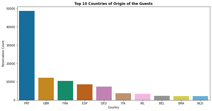
- About 40% of all bookings are created from Portugal followed by Great Britain (10%) & France (8%)
2. Which Month is the Most Occupied (Busiest) with Bookings at the Hotel
df1['arrival_date_month'].value_counts(normalize = True)
August       0.116233
July         0.106047
May          0.098760
October      0.093475
April        0.092880
June         0.091624
September    0.088014
March        0.082034
February     0.067577
November     0.056906
December     0.056789
January      0.049661
Name: arrival_date_month, dtype: float64
ordered_months = ["January", "February", "March", "April", "May", "June", "July", "August", "September", "October", "November", "December"]
df1['arrival_date_month'] = pd.Categorical(df1['arrival_date_month'], categories=ordered_months, ordered=True)
plt.figure(figsize=(12,6))
sns.countplot(x='arrival_date_month', data = df1,palette= 'viridis')
plt.title('Most Occupied (Busiest) Month with Bookings', weight='bold')
plt.xlabel('Month')
plt.xticks(rotation=45)
plt.ylabel('Reservation Count')
Text(0, 0.5, 'Reservation Count')
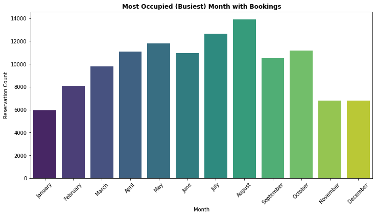
- August is the most occupied (busiest) month with 11.62% bookings and January is the most unoccupied month with 4.96% bookings.
3. How many Bookings were Cancelled at the Hotel
df1['is_canceled'].value_counts(normalize = True)
0    0.629584
1    0.370416
Name: is_canceled, dtype: float64
proportion = df1['is_canceled'].value_counts()
labels = ['Not Cancelled','Cancelled']
plt.figure(figsize=(12,6))
plt.title('Proportion of Cancelled & Not Cancelled Bookings',weight = 'bold')
plt.pie(proportion,labels=labels,shadow = True, autopct = '%1.1f%%',wedgeprops= {'edgecolor':'black'},textprops={'fontsize': 14})
plt.show()
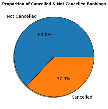
- According to the pie chart, 63% bookings were not cancelled and 37% of the bookings were cancelled at the Hotel.
4. Which Month has Highest Number of Cancellations By Hotel Type
ordered_months = ["January", "February", "March", "April", "May", "June", "July", "August", "September", "October", "November", "December"]
df1['arrival_date_month'] = pd.Categorical(df1['arrival_date_month'], categories=ordered_months, ordered=True)
plt.figure(figsize=(12,6))
sns.barplot(x = "arrival_date_month", y = "is_canceled", hue="hotel",hue_order = ["City Hotel", "Resort Hotel"],data=df1,palette= 'Blues')
plt.title("Cancelations Per Month", weight = 'bold')
plt.xlabel("Arrival Month")
plt.xticks(rotation=45)
plt.ylabel("Cancelations %")
plt.legend(loc="upper right")
plt.show()
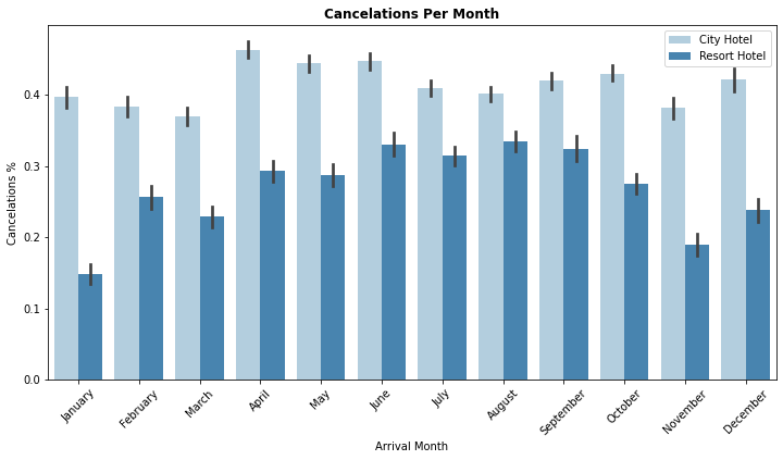
- City hotel : The number of cancelations per month is around 40% throughout the year.
- Resort hotel : The number of cancellations are highest in the summer (June,July, August) and lowest during the winter (November,December,January). In short, the possibility of cancellation for resort hotels in winter is very low.
5. How many Bookings were Cancelled by Hotel Type
df1.groupby('is_canceled')['hotel'].value_counts(normalize = True)
is_canceled  hotel
0            City Hotel      0.615012
             Resort Hotel    0.384988
1            City Hotel      0.748508
             Resort Hotel    0.251492
Name: hotel, dtype: float64
plt.figure(figsize=(12,6))
sns.countplot(x= 'is_canceled',data = df1,hue = 'hotel',palette= 'Set1')
plt.title("Cancelation Status By Hotel Type ", weight = 'bold')
plt.xlabel("Cancelation Status")
plt.ylabel(" Reservations Count")
plt.show()
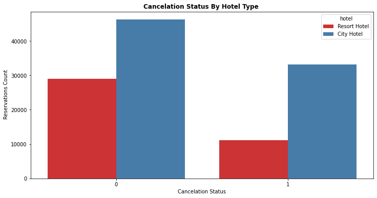
- Resort Hotel : Total of 25.14% Bookings were cancelled
- City Hotel : Total of 74.85% Bookings were cancelled
6. Relationship between Average Daily Rate(ADR) and Arrival Month by Booking cancellation status
ordered_months = ["January", "February", "March", "April", "May", "June", "July", "August", "September", "October", "November", "December"]
df1['arrival_date_month'] = pd.Categorical(df1['arrival_date_month'], categories=ordered_months, ordered=True)
plt.figure(figsize=(12,6))
sns.lineplot(x = "arrival_date_month", y = "adr", hue="is_canceled",hue_order= [1,0],data=df1,palette= 'Set1')
plt.title("Relationship between ADR and Arrival Month by Booking cancellation status", weight = 'bold')
plt.xlabel("Arrival Month")
plt.xticks(rotation=45)
plt.ylabel("Average Daily Rate")
plt.legend(loc="upper right")
plt.show()
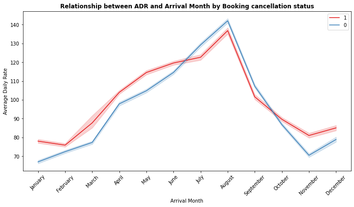
- August is the most occupied (Busiest) month of bookings.
- Highest Average Daily Rate(ADR) is in August may be it could be one of the reasons for more canceled bookings.
7. Total Number of Bookings by Market Segment
df1['market_segment'].value_counts(normalize = True)
Online TA        0.473046
Offline TA/TO    0.202856
Groups           0.165935
Direct           0.105587
Corporate        0.044350
Complementary    0.006223
Aviation         0.001985
Undefined        0.000017
Name: market_segment, dtype: float64
plt.figure(figsize=(12,6))
sns.countplot(df1['market_segment'], palette='colorblind',order=pd.value_counts(df1['market_segment']).index)
plt.title('Total Number of Bookings by Market Segment', weight='bold')
plt.xlabel('Market Segment')
plt.ylabel('Reservation Count')
Text(0, 0.5, 'Reservation Count')
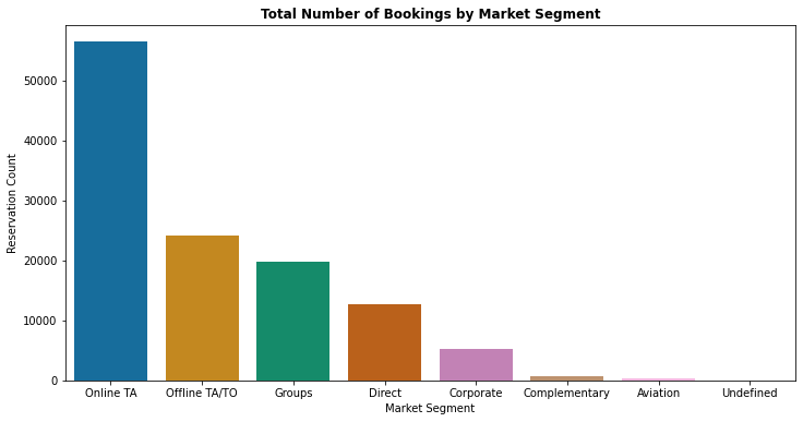
- Above graph depicts that 47.3% of bookings are made via Online Travel Agents
- Around 20% of bookings are made via Offline Travel Agents and less than 20% of bookings made directly without any Agents
8. Total Nights Spent by Guests at the Hotel by Market Segment and Hotel Type
df1['total_stay'] = df1['stays_in_week_nights'] + df1['stays_in_weekend_nights']
plt.figure(figsize=(12,6))
sns.barplot(x = "market_segment", y = "total_stay", data = df1, hue = "hotel", palette = 'rocket')
plt.title('Total Nights Spent by Guests by Market Segment & Hotel Type', weight='bold')
plt.xlabel('Market Segment')
plt.ylabel('Number of Days')
plt.legend(loc = "upper right")
<matplotlib.legend.Legend at 0x7fe1be830d10>
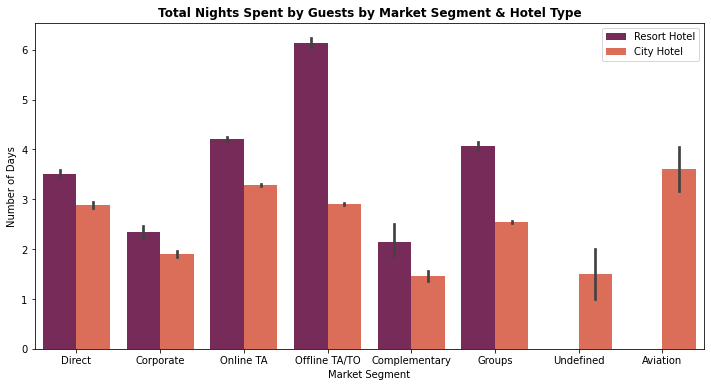
- City Hotel: Most of guests prefer to stay between 1-4 nights
- Resort Hotel : Most of the guests prefer to stay more than 3 nights
9. Arrival Date Year vs Lead Time By Booking Cancellation Status
plt.figure(figsize=(12,6))
sns.barplot(x='arrival_date_year', y ='lead_time', hue="is_canceled", data=df1, palette="viridis")
plt.title('Arrival Year vs Lead Time By Cancellation Status', weight='bold')
plt.xlabel(' Arrival Year')
plt.ylabel('Lead Time')
plt.legend(loc = "upper right")
<matplotlib.legend.Legend at 0x7fe1bcec7e10>
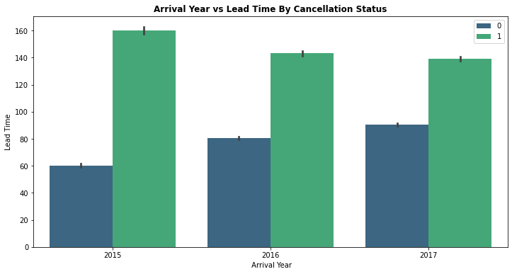
- For all the 3 years, bookings with lead time more than 100 days has more chances of getting cancelled
10. Total Number of bookings by deposit type
df1['deposit_type'].value_counts(normalize = True)
No Deposit    0.876464
Non Refund    0.122179
Refundable    0.001357
Name: deposit_type, dtype: float64
proportion = df1['deposit_type'].value_counts()
labels = ['No Deposit','Non Refundable','Refundable']
plt.figure(figsize=(12,6))
plt.title('Proportion of Total Bookings by Deposit Type',weight = 'bold')
plt.pie(proportion,labels=labels,shadow = True, autopct = '%1.1f%%',wedgeprops= {'edgecolor':'black'},textprops={'fontsize': 14})
plt.show()
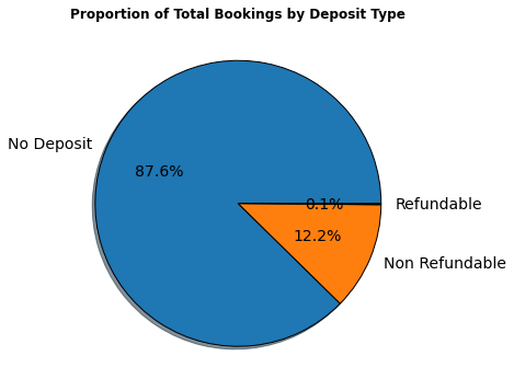
- Around 87.6% bookings are booked without deposit, 12.2% bookings are booked with Non Refundable Policy and 0.1% bookings are booked with Refundable Policy
4. Data Preparation
After exploring the dataset, we will find a lot of information that will help you prepare the data. Most important steps in Data Preparation are:
- Handling Missing Values
- Exploring Numerical and Categorical Features
- Feature Engineering (Encoding Categorical Features)
- Feature Selection (Correlation Heat Map)
4.1 Exploring Numerical Features
num_feature = [feature for feature in df1.columns if df1[feature].dtype != 'object']
print("Number of Numerical Features are : ",len(num_feature))
Number of Numerical Features are : 22
df1[num_feature][:5]
| is_canceled | lead_time | arrival_date_year | arrival_date_month | arrival_date_week_number | arrival_date_day_of_month | stays_in_weekend_nights | stays_in_week_nights | adults | children | babies | is_repeated_guest | previous_cancellations | previous_bookings_not_canceled | booking_changes | agent | company | days_in_waiting_list | adr | required_car_parking_spaces | total_of_special_requests | total_stay | |
|---|---|---|---|---|---|---|---|---|---|---|---|---|---|---|---|---|---|---|---|---|---|---|
| 0 | 0 | 342 | 2015 | July | 27 | 1 | 0 | 0 | 2 | 0.0 | 0 | 0 | 0 | 0 | 3 | NaN | NaN | 0 | 0.0 | 0 | 0 | 0 |
| 1 | 0 | 737 | 2015 | July | 27 | 1 | 0 | 0 | 2 | 0.0 | 0 | 0 | 0 | 0 | 4 | NaN | NaN | 0 | 0.0 | 0 | 0 | 0 |
| 2 | 0 | 7 | 2015 | July | 27 | 1 | 0 | 1 | 1 | 0.0 | 0 | 0 | 0 | 0 | 0 | NaN | NaN | 0 | 75.0 | 0 | 0 | 1 |
| 3 | 0 | 13 | 2015 | July | 27 | 1 | 0 | 1 | 1 | 0.0 | 0 | 0 | 0 | 0 | 0 | 304.0 | NaN | 0 | 75.0 | 0 | 0 | 1 |
| 4 | 0 | 14 | 2015 | July | 27 | 1 | 0 | 2 | 2 | 0.0 | 0 | 0 | 0 | 0 | 0 | 240.0 | NaN | 0 | 98.0 | 0 | 1 | 2 |
4.2 Exploring Categorical Features
cat_feature = [feature for feature in df1.columns if df1[feature].dtype == 'object']
print("Number of Categorical Features are : ",len(cat_feature))
Number of Categorical Features are : 12
df1[cat_feature][:5]
| _id | hotel | meal | country | market_segment | distribution_channel | reserved_room_type | assigned_room_type | deposit_type | customer_type | reservation_status | reservation_status_date | |
|---|---|---|---|---|---|---|---|---|---|---|---|---|
| 0 | 617745f32cb05b4871a1523c | Resort Hotel | BB | PRT | Direct | Direct | C | C | No Deposit | Transient | Check-Out | 2015-07-01 |
| 1 | 617745f32cb05b4871a1523d | Resort Hotel | BB | PRT | Direct | Direct | C | C | No Deposit | Transient | Check-Out | 2015-07-01 |
| 2 | 617745f32cb05b4871a1523e | Resort Hotel | BB | GBR | Direct | Direct | A | C | No Deposit | Transient | Check-Out | 2015-07-02 |
| 3 | 617745f32cb05b4871a1523f | Resort Hotel | BB | GBR | Corporate | Corporate | A | A | No Deposit | Transient | Check-Out | 2015-07-02 |
| 4 | 617745f32cb05b4871a15240 | Resort Hotel | BB | GBR | Online TA | TA/TO | A | A | No Deposit | Transient | Check-Out | 2015-07-03 |
4.3 Handling Missing Values
df1.isnull().sum()
_id                                    0
hotel                                  0
is_canceled                            0
lead_time                              0
arrival_date_year                      0
arrival_date_month                     0
arrival_date_week_number               0
arrival_date_day_of_month              0
stays_in_weekend_nights                0
stays_in_week_nights                   0
adults                                 0
children                               4
babies                                 0
meal                                   0
country                              488
market_segment                         0
distribution_channel                   0
is_repeated_guest                      0
previous_cancellations                 0
previous_bookings_not_canceled         0
reserved_room_type                     0
assigned_room_type                     0
booking_changes                        0
deposit_type                           0
agent                              16340
company                           112593
days_in_waiting_list                   0
customer_type                          0
adr                                    0
required_car_parking_spaces            0
total_of_special_requests              0
reservation_status                     0
reservation_status_date                0
total_stay                             0
dtype: int64
# Check % of Missing Values in the Data set
feature_nan = [feature for feature in df1.columns if df1[feature].isnull().sum()>1]
for feature in feature_nan:
    print('{} : {}% Missing values'.format(feature,np.around(df1[feature].isnull().mean(),4)))
children : 0.0% Missing values
country : 0.0041% Missing values
agent : 0.1369% Missing values
company : 0.9431% Missing values
- “Company” feature has almost 94% missing values. Therefore, we do not have enough values to fill the rows or Impute the company column by mean, median etc. Hence we can drop the “Company” feature.
- “Agent” feature has 13.69% missing values. “Agent” feature is travel agency Id and these values are unique and we cannot impute Id by mean, median or mode. Therefore, missing data for “Agent” can be filled by 0.
- “Country” feature has 0.4% missing values. Since missing data of “Country” is less than 1%, we can will impute with most frequent value (Mode).
- “Children” feature has only 4 missing values and we can fill these missing values by 0 considering guests have no children.
#Dropping the "Company" feature
df1.drop(columns = ['company'],inplace= True)
#Filling missing values by 0 for "Agent" feature
df1['agent']= df1['agent'].fillna(0)
#Imputing missing values of "Country" feature
df1['country'].fillna(df1['country'].mode()[0], inplace=True)
#Filling missing values by 0 for "Children" feature
df1['children']= df1['children'].fillna(0)
#Dropping the "_Id" feature
df1.drop(columns = ['_id'],inplace= True)
df2 = df1.copy()
4.4 Feature Engineering (Encoding Categorical Features)
cat_feature = [feature for feature in df2.columns if df2[feature].dtype == 'object']
print("Number of Categorical Features are : ",len(cat_feature))
Number of Categorical Features are : 11
df2[cat_feature][:5]
| hotel | meal | country | market_segment | distribution_channel | reserved_room_type | assigned_room_type | deposit_type | customer_type | reservation_status | reservation_status_date | |
|---|---|---|---|---|---|---|---|---|---|---|---|
| 0 | Resort Hotel | BB | PRT | Direct | Direct | C | C | No Deposit | Transient | Check-Out | 2015-07-01 |
| 1 | Resort Hotel | BB | PRT | Direct | Direct | C | C | No Deposit | Transient | Check-Out | 2015-07-01 |
| 2 | Resort Hotel | BB | GBR | Direct | Direct | A | C | No Deposit | Transient | Check-Out | 2015-07-02 |
| 3 | Resort Hotel | BB | GBR | Corporate | Corporate | A | A | No Deposit | Transient | Check-Out | 2015-07-02 |
| 4 | Resort Hotel | BB | GBR | Online TA | TA/TO | A | A | No Deposit | Transient | Check-Out | 2015-07-03 |
# Identify unique (Distinct) labels that exists in each categorical features
for feature in cat_feature:
    print("{} : {} labels ".format(feature,len(df2[feature].unique())))
hotel : 2 labels
meal : 5 labels
country : 177 labels
market_segment : 8 labels
distribution_channel : 5 labels
reserved_room_type : 10 labels
assigned_room_type : 12 labels
deposit_type : 3 labels
customer_type : 4 labels
reservation_status : 3 labels
reservation_status_date : 926 labels
#Custom mapping
df2['hotel'] = df2['hotel'].map({'Resort Hotel':0, 'City Hotel':1})
df2['arrival_date_month'] = df2['arrival_date_month'].map({'January':1, 'February': 2, 'March':3, 'April':4, 'May':5, 'June':6, 'July':7,
                                                            'August':8, 'September':9, 'October':10, 'November':11, 'December':12})
#Replacing "Undefined" with "SC" as mentioned in data set description
df2["meal"].replace("Undefined", "SC", inplace=True)
#Applying label encoding for categorical features
from sklearn.preprocessing import LabelEncoder
le = LabelEncoder()
df2['meal'] = le.fit_transform(df2['meal'])
df2['deposit_type'] = le.fit_transform(df2['deposit_type'])
df2['customer_type'] = le.fit_transform(df2['customer_type'])
df2['market_segment'] = le.fit_transform(df2['market_segment'])
df2['distribution_channel'] = le.fit_transform(df2['distribution_channel'])
df2['reserved_room_type'] = le.fit_transform(df2['reserved_room_type'])
df2['assigned_room_type']= le.fit_transform(df2['assigned_room_type'])
df2['reservation_status'] = le.fit_transform(df2['reservation_status'])
df2['reservation_status_date'] = le.fit_transform(df2['reservation_status_date'])
df2['country'] = le.fit_transform(df2['country'])
4.5 Feature Selection
# Relationship between Independent and Dependent feature (Correlation Heat map)
df2.corr()["is_canceled"].sort_values()
reservation_status               -0.917196
total_of_special_requests        -0.234658
required_car_parking_spaces      -0.195498
assigned_room_type               -0.176028
reservation_status_date          -0.162135
booking_changes                  -0.144381
is_repeated_guest                -0.084793
customer_type                    -0.068140
reserved_room_type               -0.061282
previous_bookings_not_canceled   -0.057358
agent                            -0.046529
babies                           -0.032491
meal                             -0.015693
arrival_date_day_of_month        -0.006130
stays_in_weekend_nights          -0.001791
children                          0.005036
arrival_date_week_number          0.008148
arrival_date_year                 0.016660
total_stay                        0.017779
stays_in_week_nights              0.024765
adr                               0.047557
days_in_waiting_list              0.054186
market_segment                    0.059338
adults                            0.060017
previous_cancellations            0.110133
hotel                             0.136531
distribution_channel              0.167600
country                           0.267502
lead_time                         0.293123
deposit_type                      0.468634
is_canceled                       1.000000
Name: is_canceled, dtype: float64
plt.figure(figsize = (15,10))
sns.heatmap(df2.corr(), cmap="viridis")
<matplotlib.axes._subplots.AxesSubplot at 0x7fe1bcde00d0>
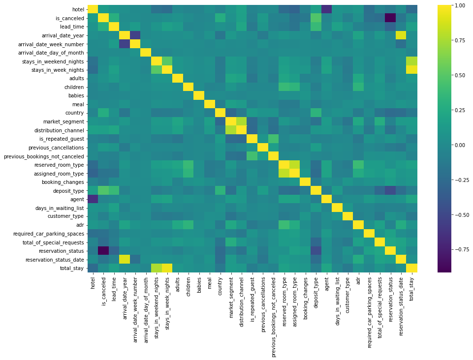
- “reservation_status” seems to be most impactful feature and because of its negative correlation with the “is_canceled” feature it can cause a wrong prediction or overfitting and there is chance of data leakage. Hence I will drop this feature.
- I will not use arrival_date_week_number, arrival_date_month, arrival_date_year,stays_in_week_nights, stays_in_weekend_nights since their importances are really low while predicting cancellations.
- “reservation_status_date” is date type data and it could not convert another type, this feature can also be dropped
df2.drop(columns = ['reservation_status','arrival_date_week_number','arrival_date_month','arrival_date_year','stays_in_week_nights','stays_in_weekend_nights','reservation_status_date'],inplace = True)
df3 = df2.copy()
df3.head()
| hotel | is_canceled | lead_time | arrival_date_day_of_month | adults | children | babies | meal | country | market_segment | distribution_channel | is_repeated_guest | previous_cancellations | previous_bookings_not_canceled | reserved_room_type | assigned_room_type | booking_changes | deposit_type | agent | days_in_waiting_list | customer_type | adr | required_car_parking_spaces | total_of_special_requests | total_stay | |
|---|---|---|---|---|---|---|---|---|---|---|---|---|---|---|---|---|---|---|---|---|---|---|---|---|---|
| 0 | 0 | 0 | 342 | 1 | 2 | 0.0 | 0 | 0 | 135 | 3 | 1 | 0 | 0 | 0 | 2 | 2 | 3 | 0 | 0.0 | 0 | 2 | 0.0 | 0 | 0 | 0 |
| 1 | 0 | 0 | 737 | 1 | 2 | 0.0 | 0 | 0 | 135 | 3 | 1 | 0 | 0 | 0 | 2 | 2 | 4 | 0 | 0.0 | 0 | 2 | 0.0 | 0 | 0 | 0 |
| 2 | 0 | 0 | 7 | 1 | 1 | 0.0 | 0 | 0 | 59 | 3 | 1 | 0 | 0 | 0 | 0 | 2 | 0 | 0 | 0.0 | 0 | 2 | 75.0 | 0 | 0 | 1 |
| 3 | 0 | 0 | 13 | 1 | 1 | 0.0 | 0 | 0 | 59 | 2 | 0 | 0 | 0 | 0 | 0 | 0 | 0 | 0 | 304.0 | 0 | 2 | 75.0 | 0 | 0 | 1 |
| 4 | 0 | 0 | 14 | 1 | 2 | 0.0 | 0 | 0 | 59 | 6 | 3 | 0 | 0 | 0 | 0 | 0 | 0 | 0 | 240.0 | 0 | 2 | 98.0 | 0 | 1 | 2 |
df3.shape
(119390, 25)
5. Modeling
-
The next step now is to build a Machine learning model using a Machine learning Algorithm. In this project, we will build Decision Tree Machine Learning Model using Scikit Learn Library.
-
We need to divide/split the data into training and test sets using train_test_split.
-
For better training of a machine learning model, it is necessary to divide the training data with more numbers (70% to 80%) of samples and the test set with 20% to 30% of the dataset depending on the size of the data.
5.1 What is Decision Tree Algorithm?
Decision tree algorithm is one of the most versatile algorithms in machine learning which can perform both classification and regression analysis. It is very powerful and works great with complex datasets. Apart from that, it is very easy to understand and read.
As the name suggests, this algorithm works by dividing the whole dataset into a tree-like structure based on some rules and conditions and then gives prediction based on those conditions. Let’s understand the approach to decision tree with a basic scenario.
Let’s assume we want to classify whether a customer could retire or not based on their savings and age.
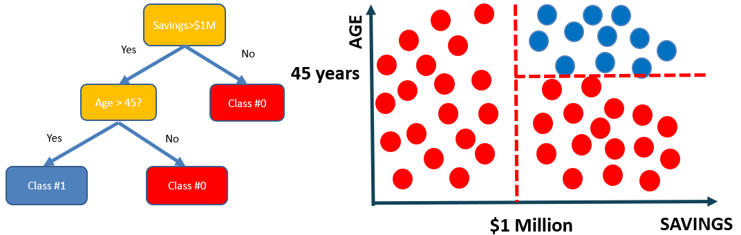
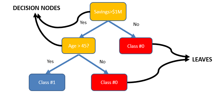
- The tree consists of decision nodes and leaves.
- Leaves are the decisions or the final outcomes.
- Decision nodes are where the data is split based on a certain attribute.
- Objective is to minimize the entropy which provides the optimum split
5.2 How does a Decision Tree Algorithm decide where to split?
Attribute Selection Measures
Attribute selection measure can be used as a basic set of rules to select the splitting criterion that helps in dividing the dataset in the best possible way. The splitting feature is always a best score attribute. Entropy, Information Gain, Gini Index and Gain Ratio are the most commonly used and popular selection measures.
Entropy
Entropy is the measure of randomness in the data. In other words, it gives the impurity present in the dataset.
When we split our nodes into two regions and put different observations in both the regions, the main goal is to reduce the entropy i.e. reduce the randomness in the region and divide our data cleanly than it was in the previous node. If splitting the node doesn’t lead into entropy reduction, we try to split based on a different condition, or we stop.
A region is clean (low entropy) when it contains data with the same labels and random if there is a mixture of labels present (high entropy).
Let’s suppose there are ‘m’ observations and we need to classify them into categories 1 and 2. Let’s say that category 1 has ‘n’ observations and category 2 has ‘m-n’ observations.
p= n/m and q = m-n/m = 1-p
then, entropy for the given set is:
E = -plog2(p) – qlog2(q)
When all the observations belong to category 1, then p = 1 and all observations belong to category 2, then p =0, int both cases E =0, as there is no randomness in the categories.
If half of the observations are in category 1 and another half in category 2, then p =1/2 and q =1/2, and the entropy is maximum, E =1.
Information Gain
Information gain calculates the decrease in entropy after splitting a node. It is the difference between entropies before and after the split. The more the information gain, the more entropy is removed.
Constructing a decision tree is all about finding an attribute that returns the highest information gain and the smallest entropy.
Mathematically, IG is represented as:
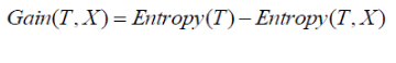
Where, T is the parent node before split and X is the split node from T.
Gini Index
Gini index is a cost function used to evaluate splits in the dataset. It is calculated by subtracting the sum of the squared probabilities of each class from one. It favors larger partitions and easy to implement whereas information gain favors smaller partitions with distinct values.
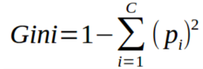
Steps to Calculate Gini for a split
- Calculate Gini for sub-nodes, using the formula sum of the square of probability for success and failure (p^2+q^2).
- Calculate Gini for split using weighted Gini score of each node of that split
5.3 Decision Tree Implementation in Python
X = df3.drop(['is_canceled'], axis = 1)
y = df3['is_canceled']
#Train and test split data
from sklearn.model_selection import train_test_split
X_train,X_test,y_train,y_test = train_test_split(X,y,random_state = 42,stratify = y,test_size = 0.30)
#Checking if train and test data of target feature is equally distributed
y_train.value_counts(normalize=True)
0    0.629581
1    0.370419
Name: is_canceled, dtype: float64
y_test.value_counts(normalize=True)
0    0.629589
1    0.370411
Name: is_canceled, dtype: float64
5.4 Model Training
Steps to be followed to build Machine Learning Model with Scikit-learn
- Import and choose the classifier you plan to use
- Instantiate the Estimator
- Fit the model with data
- Predict the Target feature for a new observation
# import the class
from sklearn.tree import DecisionTreeClassifier

# instantiate the estimator(model)
dt_model = DecisionTreeClassifier(random_state = 42)

#fit the model with data
dt_model.fit(X_train,y_train)
DecisionTreeClassifier(ccp_alpha=0.0, class_weight=None, criterion='gini',
                       max_depth=None, max_features=None, max_leaf_nodes=None,
                       min_impurity_decrease=0.0, min_impurity_split=None,
                       min_samples_leaf=1, min_samples_split=2,
                       min_weight_fraction_leaf=0.0, presort='deprecated',
                       random_state=42, splitter='best')
#Predict the Target feature for a new observation
dt_model.predict(X_train)
array([1, 0, 0, ..., 0, 1, 0], dtype=int64)
#Accuracy score on Training Data
dt_model.score(X_train,y_train)
0.996434255082383
-
The training set accuracy is close to 100%! But we can’t rely solely on the training set accuracy, we must evaluate the model on the test data set too.
-
We can make predictions and compute accuracy in one step using model.score
#Accuracy score on Testing Data
dt_model.score(X_test,y_test)
0.8441242985174637
- It appears that the model has learned the training data perfect (99%), and doesn’t generalize well to previously unseen data (84%). This is called overfitting, and reducing overfitting is one of the most important parts of any machine learning project.
5.5 Visualizing Decision Trees
from sklearn.tree import plot_tree, export_text
plt.figure(figsize=(80,20))
plot_tree(dt_model, feature_names=X_train.columns, max_depth=2, filled=True)
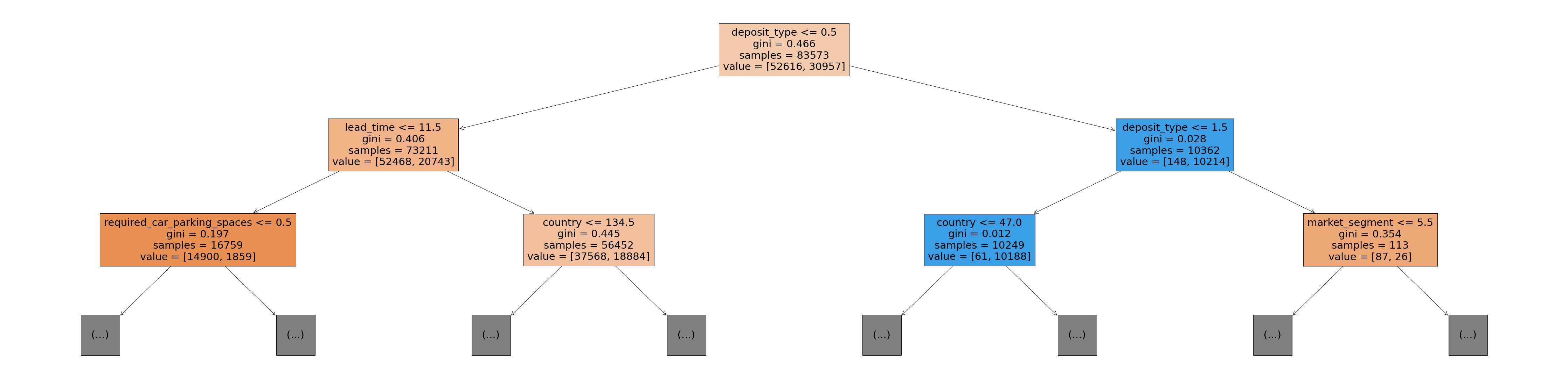
-
The Gini value in each box is the loss function used by the decision tree to decide which column should be used for splitting the data, and at what point the column should be split.
-
Lower Gini index indicates a better split
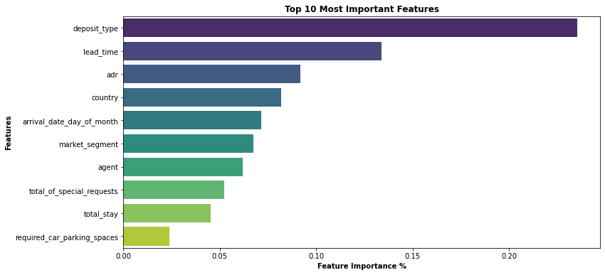
5.6 Feature Importance
Based on the Gini Index computations, a decision tree assigns an “importance” value to each feature. These values can be used to interpret the results given by a decision tree.
dt_model.feature_importances_
array([0.00430979, 0.13396326, 0.0714008 , 0.01165362, 0.00543306,
       0.00069664, 0.01043204, 0.08195502, 0.06748312, 0.00350234,
       0.00182046, 0.02199886, 0.00573351, 0.01277278, 0.01703412,
       0.0153714 , 0.23543993, 0.06189516, 0.00334881, 0.02076981,
       0.09174907, 0.02378499, 0.05232125, 0.04513017])
#Convert this into a dataframe and visualize the most important features
importance_df = pd.DataFrame({
    'feature': X_train.columns,
    'importance': dt_model.feature_importances_
}).sort_values('importance', ascending=False)
plt.figure(figsize=(12,6))
sns.barplot(data=importance_df.head(10), x='importance', y='feature',palette= 'viridis')
plt.title('Top 10 Most Important Features', weight='bold')
plt.xlabel('Feature Importance %',weight='bold')
plt.ylabel('Features',weight='bold')
Text(0, 0.5, 'Features')
5.7 Model Evaluation
-
We can increase the model performance by hyperparameter tuning and finding these optimal hyperparameters would help us achieve the best-performing model.
-
GridSearchCV uses a different combination of all the specified hyperparameters and their values and calculates the performance for each combination and selects the best value for the hyperparameters. This will cost us the processing time and expense but will surely give us the best results.
-
Cross Validation is a statistical method used to estimate the performance (or accuracy) of Machine learning Models. It is used to protect against overfitting in a predictive model.
# Hyper Parameter Tuning using Grid SeachCV on Decision Tree Algorithm to check Best score and Best parameters

from sklearn.model_selection import GridSearchCV

param_grid= { 'criterion' : ['gini', 'entropy'],'min_samples_split' : [2,4,6,8],
                  'min_samples_leaf': [1,2,3,4,5],'max_features' : ['auto', 'sqrt'],'max_depth': [1,2,3,4,5,6,7,8,9,10]}

clf = GridSearchCV(estimator=dt_model, param_grid = param_grid, cv = 10, n_jobs=-1)
best_clf = clf.fit(X_train,y_train)
print('Decision Tree Best score: {} using best parameters {}'.format(best_clf.best_score_, best_clf.best_params_))
Decision Tree Best score: 0.8155264977113239 using best parameters {'criterion': 'gini', 'max_depth': 10, 'max_features': 'auto', 'min_samples_leaf': 1, 'min_samples_split': 6}
- Best score is 0.8155264977113239
- Best parameters are {‘criterion’: ‘gini’, ‘max_depth’: 10, ‘max_features’: ‘auto’, ‘min_samples_leaf’: 1, ‘min_samples_split’: 6}
# Stratified K-fold Cross Validation Technique on Decision Tree Alogorithm to know the exact Mean CV accuracy score
# Impute the best parameters obtained in Hyper Parameter tuning for Decision Tree Algorithm

from sklearn.model_selection import cross_val_score,StratifiedKFold
skfold = StratifiedKFold(n_splits= 10,shuffle= True,random_state= 42)

dt_cv_result = cross_val_score(DecisionTreeClassifier(criterion = 'gini',max_depth = 10, max_features = 'auto', min_samples_leaf = 1,min_samples_split = 6),X, y, cv=skfold,scoring="accuracy",n_jobs=-1)
dt_cv = dt_cv_result.mean()*100
print('Decision Tree CV Mean Accuarcy Score is {}'.format(dt_cv))
Decision Tree CV Mean Accuarcy Score is 80.52935756763547
-
Optimizing Decision Tree Model Performance
-
Impute the best parameters obtained in Hyper Parameter tuning for the newly created Decision Tree model to obtain Best Accuracy Score
# instantiate the estimator(new model)
dt_model_new = DecisionTreeClassifier(random_state = 42,criterion = 'gini',max_depth = 10, max_features = 'auto',
                                      min_samples_leaf = 1,min_samples_split = 6)

#fit the new model with data
dt_model_new.fit(X_train,y_train)
DecisionTreeClassifier(ccp_alpha=0.0, class_weight=None, criterion='gini',
                       max_depth=10, max_features='auto', max_leaf_nodes=None,
                       min_impurity_decrease=0.0, min_impurity_split=None,
                       min_samples_leaf=1, min_samples_split=6,
                       min_weight_fraction_leaf=0.0, presort='deprecated',
                       random_state=42, splitter='best')
#Accuracy score on Training Data
dt_model_new.score(X_train,y_train)
0.8099146853648905
#Accuracy score on Test Data
dt_model_new.score(X_test,y_test)
0.8047854370829495
- It appears that the model has learned the training data perfect (80.99%), and it generalizes well on test (unseen) data (80.47%)
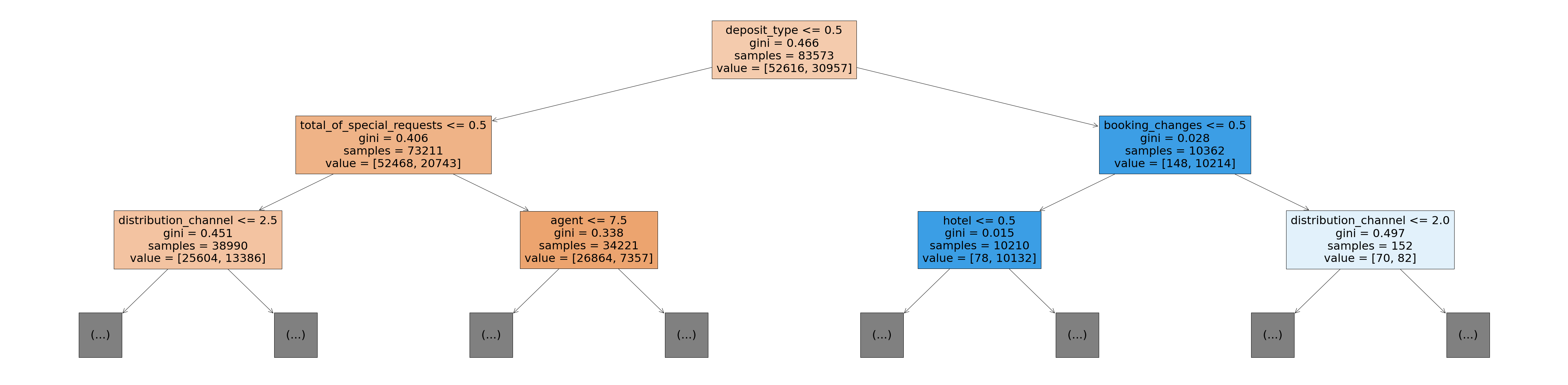
# Visualizing Optimized Decision Tree
plt.figure(figsize=(80,20))
plot_tree(dt_model_new, feature_names=X_train.columns, max_depth=2, filled=True)
# Since the size of the pickle file is more, I will compress the pickle file using BZ2 library**
import bz2,pickle
sfile = bz2.BZ2File('dt_model_new_pickle.pkl','wb')
pickle.dump(dt_model_new,sfile)
sfile.close()
df4 = df3.copy()
df4.head()
| hotel | is_canceled | lead_time | arrival_date_day_of_month | adults | children | babies | meal | country | market_segment | distribution_channel | is_repeated_guest | previous_cancellations | previous_bookings_not_canceled | reserved_room_type | assigned_room_type | booking_changes | deposit_type | agent | days_in_waiting_list | customer_type | adr | required_car_parking_spaces | total_of_special_requests | total_stay | |
|---|---|---|---|---|---|---|---|---|---|---|---|---|---|---|---|---|---|---|---|---|---|---|---|---|---|
| 0 | 0 | 0 | 342 | 1 | 2 | 0.0 | 0 | 0 | 135 | 3 | 1 | 0 | 0 | 0 | 2 | 2 | 3 | 0 | 0.0 | 0 | 2 | 0.0 | 0 | 0 | 0 |
| 1 | 0 | 0 | 737 | 1 | 2 | 0.0 | 0 | 0 | 135 | 3 | 1 | 0 | 0 | 0 | 2 | 2 | 4 | 0 | 0.0 | 0 | 2 | 0.0 | 0 | 0 | 0 |
| 2 | 0 | 0 | 7 | 1 | 1 | 0.0 | 0 | 0 | 59 | 3 | 1 | 0 | 0 | 0 | 0 | 2 | 0 | 0 | 0.0 | 0 | 2 | 75.0 | 0 | 0 | 1 |
| 3 | 0 | 0 | 13 | 1 | 1 | 0.0 | 0 | 0 | 59 | 2 | 0 | 0 | 0 | 0 | 0 | 0 | 0 | 0 | 304.0 | 0 | 2 | 75.0 | 0 | 0 | 1 |
| 4 | 0 | 0 | 14 | 1 | 2 | 0.0 | 0 | 0 | 59 | 6 | 3 | 0 | 0 | 0 | 0 | 0 | 0 | 0 | 240.0 | 0 | 2 | 98.0 | 0 | 1 | 2 |
df4.shape
(119390, 25)
6. Model Deployment
-
After building a model, the final stage of the machine learning lifecycle is to deploy the ML model.
-
ML model should be scalable and accessible to the business users/Customers by creating Web Application and deploying the model on the cloud using AWS, Google Cloud, Heroku cloud platforms.
-
Inorder to build the Web app, I will use the 10 most important features that are helpful in predicting the Hotel Booking Cancelation from the guests since it would be pain to front end user to fill all 23 features on the web app. I will drop the rest of features so we can build an interactive and user friendly web app
X = df4.drop(['is_canceled','hotel','arrival_date_day_of_month','adults','children','babies','meal','country','distribution_channel','is_repeated_guest',
              'previous_bookings_not_canceled','reserved_room_type','agent','days_in_waiting_list'],axis = 1)
y = df4['is_canceled']
#Train and test data again to check if there is any drop in accuracy of the model after eliminating features
from sklearn.model_selection import train_test_split
X_train,X_test,y_train,y_test = train_test_split(X,y,random_state = 42,stratify = y,test_size = 0.30)
from sklearn.tree import DecisionTreeClassifier
dt_model_new = DecisionTreeClassifier(random_state = 42)
dt_model_new.fit(X_train,y_train)
DecisionTreeClassifier(ccp_alpha=0.0, class_weight=None, criterion='gini',
                       max_depth=None, max_features=None, max_leaf_nodes=None,
                       min_impurity_decrease=0.0, min_impurity_split=None,
                       min_samples_leaf=1, min_samples_split=2,
                       min_weight_fraction_leaf=0.0, presort='deprecated',
                       random_state=42, splitter='best')
dt_model_new.score(X_train,y_train)
0.987675445418975
dt_model_new.score(X_test,y_test)
0.8125191947957674
# Compress the Pickle file to store Machine Learning Model for Web App Development
import bz2,pickle
file = bz2.BZ2File('dtmodelfinal.pkl','wb')
pickle.dump(dt_model_new,file)
file.close()
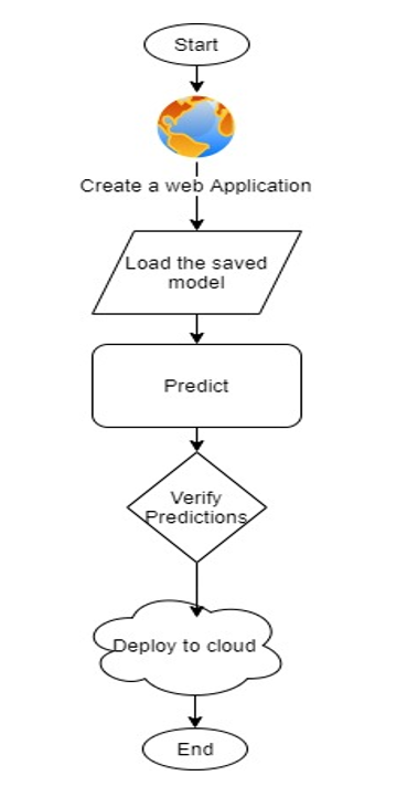
6.1 Machine Learning Web App Deployment on Heroku Cloud Using Python & Streamlit
Once the training is completed, we need to expose the trained model as an API for the user to consume it. For prediction, the saved model is loaded first and then the predictions are made using it. If the web app works fine, the same app is deployed to the cloud platform.
ML Application flow chart
6.2 ML Web App Demonstration Video
Link to the ML Web app :
https://cancelation-predictor.herokuapp.com/
Link for Python Code available on GitHub :
6.3 Video Demonstration of Machine Learning Project
Summary
From our Data Analysis, we have observed that the top 5 most important features in the data set which helps in predicting hotel cancellations from the guests are :
- Lead Time
- Average Daily Rate (ADR)
- Deposit Type
- Arrival Day of the Month
- Country
Strategies to Counter High Cancellations at the Hotel
- Set Non-refundable Rates, Collect deposits, and implement more rigid cancellation policies.
- Using Advanced Purchase Rates with varying Lead Time windows
- Encourage Direct bookings by offering special discounts
- Hotels should consider the total number of special requests from guests to reduce the possibility of cancellations by improving customer service.
- Monitor where the cancellations are coming from such as Market Segment, distribution channels, etc.
References
- https://www.pegs.com/blog/how-hotels-can-counter-high-ota-cancellation-rates/
- https://www.d-edge.com/how-online-hotel-distribution-is-changing-in-europe/
- https://www.kaggle.com/jessemostipak/hotel-booking-demand